
Monitoring the quality and quantity of training and competition stress is essential to understanding the dose-response relationship of physiological and biomechanical loads and adaptations. This information informs decision making in training periodization, reverse engineering the physical demands of a sport, and managing training stress during the season to ensure athletes are physically peaking for competition.
GPS units are the most common tool for measuring training stress in American football. The demands of American football are common to most field based team sports: a mix of sprinting, high speed running, and multi-directional movements; a range of position specific demands; and movements and actions in both large and small spaces. In addition to running based metrics, such as distances travelled within velocity bands, GPS devices also provide metrics that differentiate running activities from non-running activities such as collisions, impacts, and changes of direction and movement tasks that produce very little body movement in small spaces[1].
This article will focus on GPS metrics that help us understand external load – the physical work athletes perform during sport – and how we can detect relevant changes in that data.
Tweet ThisMonitoring the quality and quantity of training and competition stress is essential to understanding the dose-response relationship of physiological and biomechanical loads and adaptations
@marctlewis
Selecting from a menu of metrics
The most appropriate metrics will represent the physical demands of the position, demonstrate an adequate level of reliability, and capture different training constructs related to stress.
| Category | Definition | Examples |
| Volume | Total work regardless of the level of difficulty | Player load, total distance, total contacts, total throws |
| Intensity | Work above a specific band or threshold | IMAs >3.5 m/s2, impacts >7.5 g,accelerations >4.0 m/s2 |
| Density | Work per unit of time | Distance / minute, player load / minute, IMAs / minute |
| Performance | Representation of the athlete’s maximal output | Maximal acceleration, max deceleration, max velocity |
Volume
A volume metric represents the amount of work a player performs without factoring in the level of difficulty of the work. A commonly tracked volume metric is player load, which is the square root of the sum of the squared instantaneous rate of change in acceleration on the three axes, divided by 100.[3]
Player load captures both running and non-running activity, making it suitable for collision based sports that feature a variety of impacts and movement demands [3]. While the player load metric is a continuous, time dependent value, it can be adapted as an intensity metric through effort bands with pre-set thresholds[4].
Other volume indicators especially relevant to American football include total contacts and total throws.
Intensity
While a volume metric indicates total work without factoring in the level of difficulty, an intensity indicator quantifies work above a pre-established intensity threshold. These can be displayed as intensity bands with qualitative descriptors such as high, moderate, and low intensity.
Intensity bands can be set as absolute or relative to the individual (e.g., as a percentage of a maximal output). For example, acceleration bands can be based on absolute values as low < 1.49 m/s2, moderate = 1.50-2.49 m/s2, and high > 3.5 m/s2 [5].
Running bands, on the other hand, generally have both absolute and relative applications.
Relative running bands may be high velocity > 85% Vmax, moderate velocity = 70-85% Vmax, and low velocity running = 55-70% Vmax. These could apply across the whole squad, while within each position group, absolute values determine the band. Skill position players in American football may have bands of >18 mph, 15-17.99 mph, and 12-14.99 mph for high, moderate, and low, respectively.
Other intensity indicators especially relevant to American football include inertial measurement analysis, impacts, and decelerations.
Density
Density indicators describe the work completed per unit of time. A simple rule of thumb is to select the most relevant volume and intensity indicator that is consistently monitored for each group and track its density.
The most common density measure in American football is player load per minute. However, having a comprehensive understanding of the density across a range of intensity indicators will assist in off season preparation and during the rehabilitation process when preparing an athlete to return to football.
Performance
Finally, performance indicators are maximal physical outputs for a given measure. The most common in American football is maximal velocity. However, other commonly tracked performance outputs include maximal acceleration and deceleration.
During rehabilitation, the requirement for an athlete to demonstrate a percentage of their maximal output may be a criterion for progression. Otherwise, practitioners may track maximal outputs to evaluate athlete development over the course of a year.
Tweet ThisDensity indicators describe the work completed per unit of time. A simple rule of thumb is to select the most relevant volume and intensity indicator that is consistently monitored for each group and track its density
@marctlewis
Z-scores reveal meaningful changes in GPS metrics
For GPS metrics to inform decision making, we need a system to detect changes in each metric that can alert us to when an athlete is experiencing something outside of their normal dose of training stress. The system must be able to detect changes in training stress at the individual, positional, and team level. This requires an understanding of the normal distribution of values for each metric both within and between players.
Measures of central tendency and variability are excellent places to start quantifying a normal dose of training stress at the individual, positional, and team levels. Measures of central tendency and variability offer a better understanding of how likely (or unlikely) it is that an athlete experiences a given value, e.g., some volume of high speed running yards or sprinting efforts, or a threshold magnitude of acceleration or deceleration. They also can detect the magnitude of change based on the distribution of values. In general, a higher than average value represents a greater stressor to the system, resulting in a greater disturbance of homeostasis.
| Meaningful Change | Values beyond +/- 2 z-scores |
| Potentially Meaningful Change | Values between +/- 1-2 z-scores |
| Average | Values within +/- 1 z-score |
Z-scores are a simple and effective way to quickly identify values that are outside of the normal range of expected values [7]. In this case, they will quickly identify athletes who are experiencing a unusual dose of training stress. Z-scores can be calculated in a variety of ways to detect change, and can be based on daily or weekly values. Practitioners can adjust the time frame of the rolling values based on factors like time of year and the practice schedule.
Daily Z-Score = (current day metric value – daily metric rolling average) / daily metric rolling standard deviation
The daily z-score identifies athletes experiencing a meaningful change in a load metric for that day, compared to their daily average in the metric. The current daily value represents the acute load separate from the daily average of the value representing the chronic load.
Weekly Z-Score = (weekly metric value – weekly metric rolling average) / weekly metric rolling standard deviation
The weekly z-score identifies athletes experiencing a meaningful change in a load metric for the week. American football normally features one game per week, so a weekly z-score would identify athletes experiencing a meaningful change in training stress in the practices leading up to, and including, the game.
Table 3 shows athlete data over the course of a season. The athlete maintains a relatively constant player load measure (z-score = 0.11). However, measures of running distance at moderate velocity bands and higher velocity bands have been steadily increasing, with weekly z-scores of 1.02 and 2.18, respectively. These flag the athlete as having experienced a meaningful load change in his high velocity running distance.
| Season Code | Player Load | Player Load High | Low Velocity Distance | Moderate Velocity Distance | High Velocity Distance |
| REG-07-OPP-3 | 219 | 18 | 230 | 101 | 48 |
| REG-07-OPP-1 | 161 | 20 | 242 | 89 | 26 |
| REG-06-OPP-6 | 686 | 45 | 381 | 241 | 95 |
| REG-06-OPP-4 | 217 | 5 | 310 | 73 | 0 |
| REG-06-OPP-3 | 332 | 43 | 272 | 63 | 36 |
| REG-06-OPP-1 | 179 | 13 | 133 | 89 | 7 |
| REG-05-OPP-5 | 491 | 49 | 109 | 51 | 11 |
| REG-05-OPP-4 | 302 | 47 | 338 | 88 | 35 |
| REG-05-OPP-3 | 321 | 10 | 207 | 119 | 0 |
| REG-05-OPP-1 | 116 | 43 | 148 | 34 | 0 |
| REG-04-OPP-5 | 351 | 12 | 169 | 37 | 19 |
| REG-04-OPP-4 | 219 | 60 | 204 | 34 | 19 |
| REG-04-OPP-3 | 255 | 37 | 467 | 119 | 0 |
| REG-03-OPP-5 | 464 | 11 | 271 | 99 | 5 |
| REG-03-OPP-3 | 266 | 25 | 192 | 59 | 20 |
| REG-03-OPP-1 | 157 | 69 | 209 | 43 | 0 |
| REG-03-OPP-5 | 517 | 70 | 436 | 100 | 7 |
| REG-03-OPP-4 | 406 | 45 | 308 | 68 | 13 |
| REG-03-OPP-3 | 331 | 47 | 230 | 62 | 0 |
| REG-03-OPP-2 | 304 | 38 | 176 | 36 | 4 |
| REG-03-OPP-1 | 175 | 20 | 210 | 68 | 15 |
| 7 Day Average | 312 | 28 | 240 | 101 | 32 |
| 14 Day Average | 299 | 38 | 255 | 69 | 9 |
| 14 Day SD | 114 | 20 | 98 | 31 | 10 |
| Weekly Z-Score | 0.11 | -0.52 | -0.15 | 1.02 | 2.18 |
Calculating these z-scores require a rolling average and a rolling standard deviation, which we can graph and analyze separately. A rolling average is useful with training load data given the systematic pattern and random noise within these data over time. Line or bar graphs are particularly useful for displaying rolling measures of central tendency and variability. These visualizations make it easier to assess chronic change in training load, and to identify patterns within specific time frames [8]
Z-scores are a unitless, standardized measure, so they can be added, subtracted, or averaged. A composite z-score can help compare an individual to their norm at a snapshot in time, e.g., MD-3 this week vs. where they normally are at MD-3. This lets us monitor an athlete’s daily accumulation of training load throughout a week with reference to their average loads for each day and each week. For example, a player has a MD-4 with sprinting yardage z-score = .50 above normal. Based on this value, the practitioners can determine and possibly adjust his MD-3 sprinting yardage so he stays within his normal weekly total (+/- 1 SD). If the athlete’s MD-3 sprint yardage subsequently has z-score = -1.00, his weekly composite z-score is now -.50.
Z-scores from different metrics can also be summed to give a more comprehensive view of how much training stress an athlete experienced in a given time frame compared to their norm. [9]
Composite Z-Score = sum of daily z-scores for a given metric.
Data-informed individual workload prescriptions
Determining individual loading prescriptions is primarily based on the physical demands of the sport, the time frame you have to prepare the athlete for the demands, and the athlete’s individual response and tolerance to loading.
In American football, the athlete’s position weighs heavily on physical demand. A cornerback who plays only on defense will have a different physical demand than a cornerback who also plays gunner on special teams. Nuances of a position group and scheme will also result in differing physical demands. Different linebackers may serve different roles (e.g., Sam, Mike, Whip). These roles within their position group will shape whether they are covering offensive players in space, or whether they are primarily playing in the box to stop the run – tasks with very different physical demands [6].
Tweet ThisProgressing an athlete to extremely high workloads that they may only encounter once per season comes with a variety of opportunity costs: time spent not training other qualities, fatigue, and increased risk of injury during training and practice
@marctlewis
Preparing (without over-preparing) for the worst case scenario
Athletes must be prepared to handle not only their usual, in-game averages, but also the prospect of abnormal physical workloads. Many times, practitioners will plan around an athlete’s “worst case scenario.”
The worst case scenario is generally the highest physical workload an athlete may experience within a given metric. However, progressing an athlete to extremely high workloads that they may only encounter once per season comes with a variety of opportunity costs: time spent not training other qualities, fatigue associated with higher workload training interfering with the time spent training other qualities, increased risk of injury during training and practice. Worst case scenario training may also simply be impractical based on the time frame allotted and incremental progressions.
Game data is at the heart of worst case scenario training. Descriptive measures of central tendency and variability allow practitioners to understand average physical workloads across relevant metrics, along with the normal variability across a season. The baseline data could be for each individual athlete, or aggregated from players in that position.
Using this information, practitioners can prepare athletes for the physical workloads they are most likely to face, and then extrapolate the extreme (if unlikely) situations they could encounter. Then they can decide matters of practicality, prioritization, and programming.
Table 5 shows the worst case bounds using aggregated athlete data for athletes filling the roles of a cornerback on defense and a special teams gunner.
| Cornerback / gunner weekly moderate velocity running distance | |||
| Weekly code | Player X | Player Y | Player Z |
| POST-01-OPP | 324 | 652 | 552 |
| REG-16-OPP | 502 | 851 | 662 |
| REG-15-OPP | 376 | 1121 | 527 |
| REG-14-OPP | 540 | 920 | 921 |
| REG-14-OPP | 665 | 459 | 458 |
| REG-13-OPP | 518 | 652 | 542 |
| REG-12-OPP | 844 | 625 | 483 |
| REG-11-OPP | 416 | 520 | 682 |
| REG-10-OPP | 407 | 429 | 519 |
| REG-09-OPP | 553 | 501 | 652 |
| REG-08-OPP | 764 | 685 | 714 |
| REG-07-OPP | 689 | 478 | 574 |
| REG-06-OPP | 391 | 297 | 385 |
| REG-05-OPP | 222 | 770 | 958 |
| REG-04-OPP | 305 | 293 | 582 |
| REG-03-OPP | 584 | 360 | 485 |
| REG-02-OPP | 774 | 356 | 621 |
| REG-01-OPP | 757 | 429 | 478 |
| Season average (68.2% of outcomes) | 571 | 383 – 759 yards | |
| Season SD | 188 | ||
| Adverse scenario (13.6%) | 759 | 759 – 947 yards | |
| Extreme case (2.1%) | 947 | 947 – 1135 yards | |
| Worst case (<1%) | 1135 | >1135 yards | |
The range of workloads are based on the likelihood of the athlete experiencing a weekly value of moderate velocity running distance based on the sample data, assuming a normal distribution of data.
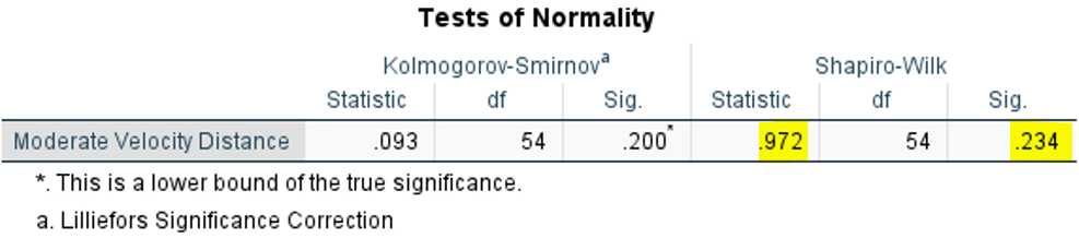
The dispersion and normality of the data can be examined using confidence intervals and testing for normality using a test such as the Shapiro-Wilk test. We can view the dispersion of the data using a histogram chart with a distribution curve (Figure 1). Figure 3 shows the output from tests of normality.
In the Shapiro-Wilk test of normality (recommended with small datasets), the W statistic is 0.972 with a significance of .234. A W statistic closer to 1 indicates with a p-value > 0.05, indicating that the data is normally distributed.

Tweet ThisDescriptive measures of central tendency and variability allow practitioners to understand average physical workloads across relevant metrics, along with the normal variability across a season
@marctlewis
In season practice planning
Before the start of the season, practitioners should collaborate with the coaching staff to develop a practice structure that considers the staff’s preference around technical skills, their tactical agenda and scheme installation, and practice structure. Practitioners should also determine how the coaching staff wants to receive information about intervention points at the team, positional, and individual levels.
There is a large degree of variation in how practice plans are structured based on the preference of the coach and level of play (e.g., NFL, college, high school). The most appropriate practice schedule will differ based on the people and context. However, there are principles that apply to any practice schedule and training methods to maximize performance and availability. These include undulation of practice loading, combining similar stressors, and organizing a practice script around the tactical and loading foci of the day.
Tweet ThisBefore starting the season, practitioners should collaborate with the coaching staff to develop a practice structure that considers the staff’s preference around technical skills, their tactical agenda and scheme installation, and practice structure
@marctlewis
| Tactical code | MD+1 | MD+2 | MD-4 | MD-3 | MD-2 | MD-1 | Game Day |
| Loading focus | Recovery | Regeneration | Game strength | Game endurance | Game speed | Recovery | Peaking |
| Tactical focus | Corrections | Plan install | Technical skills, collision, tackling | Team periods, moving the ball situations, higher speeds and faster tempos | Team periods, special teams situational, and special situation | Review assignments, situational awareness, and refine tactical plan | Execute game plan |
| Practice script considerations | Review previous game | Coaching staff finalizes game plan and plans week install | 3rd down, goal line, redzone 1-on-1s, short yardage situations on a condensed field | Kick-off coverage / kick-off return with full speed reps, open field 1-on-1s, normal downs and passing situations with a full field | Mixed team periods, punt coverage and return with release only, execute special situations at game speed | Review in walkthrough | Competition |
| Physical focus | Rest | Regeneration: soft tissue work, mobility, blood flow promotion | Strength, primary lower body lift | Strength, primary upper body lift | Speed / rate of force development; | Recovery | Potentiation medicine ball throws, plyometrics (low volume and density) |
| full body | |||||||
| Duration (min) | 50 | None | 90 | 80 | 70 | 50 | Game |
| Equipment | Jerseys only | None | Full pads | Full pads | Helmets / spiders | Helmets only | Full pads |
| Estimated average player load | 150 | None | 450 | 400 | 350 | 150 | 600 |
| Loading parameters | Minimal high intensity actions; monitor player load bands and high intensity running metrics | None | Accelerations, decelerations, collisions, impacts, high IMAs | Distance at specific velocity bands, number of efforts at specific velocity bands, high IMAs (bigs) | Distance at specific velocity bands, number of efforts at specific velocity bands, high IMAs (bigs) | Minimal high intensity actions; monitor player load bands and high intensity running metrics | All relevant metrics compared to their game norms |
| % game load | 15-25% | None | 65-75% | 55-65% | 45-55% | 15-25% | 100% |
| Other considerations | No high speed exposures or high intensity actions | Active recovery options offered and encouraged | Smaller field with highest amount of IMAs and accel / decel efforts | Large field with highest amount of high-speed yardage and sprinting efforts | Moderate to large field space with exposures to high intensity actions but limited in volume | Focus on hydration, travel tips if away, and proper fueling heading into game day | Determine weekly loading goals based on game outputs of individual athletes |
| Longer rest periods to keep density low | Longer rest periods to keep density low | Increased density of work | Moderate rest periods to reduce cardiovascular demand | ||||
Within this game week example, the row displaying “targeted loading parameters” gives examples of metrics that would represent the most significant physical demands of the day. While these illustrate the loading and tactical foci of the day, practitioners should be monitoring the metrics specific to the physical demands of the position group. Since MD-3 involves a higher volume of running based activities, the intensity of running distance at different velocity bands emerges as a priority metric. However, it might be more appropriate to monitor linemen through inertial movement analysis (IMAs), which uses the other instruments within the GPS unit (accelerometer, gyroscope, and magnetometer) to quantify acceleration forces in specific directions. [1] The IMAs can then be categorized into bands based on the rate of acceleration and used as intensity indicators.
Ultimately, the goal when using GPS units to monitor training stress is to make the information actionable to inform decision making to maximize performance and availability. This requires that we purposefully collect the data, analyze the most appropriate metrics, and then communicate those data effectively to all key stakeholders.
Tweet ThisThe goal of using GPS to monitor training stress is to make the data actionable, informing decisions to maximize performance and availability. This requires purposeful data collection, analyzing key metrics, and effectively communicating findings to stakeholders
@marctlewis