
Resilient athletes can endure and recover quickly from difficult conditions. They are mentally and physically strong, adaptable, and difficult to keep down. As such, the primary objective of performance practitioners is the development of physical and mental strength and capacity in several areas. This requires a proactive mindset that focuses on aspects within your control to prepare for multiple situations ahead of time.
However, most organisations inadvertently gravitate towards training monitoring processes that highlight when players might be at their weakest, with the view of modifying training programs or, in extreme cases, limiting playing minutes. This approach involves a reactive mindset, where practitioners have some level of anxiety or fear that a player may sustain an injury.
I have previously discussed how my incorrect use of language contributed to reactive mindsets [1]. My purpose here is to discuss some of the aspects that are important for proactive planning and monitoring in field based team sports, using the typical electronic performance and tracking systems: GPS, LPS, or semi-automatic multiple camera technology. The primary goal of this monitoring should be developing resilient players that are comfortable during the most difficult conditions they may confront in their sport.

Selecting useful training outputs that tell you something different
Thousands of external workload parameters are available to team sport practitioners via multiple software and hardware providers [2]. This creates challenges in developing monitoring processes, as practitioners may feel the need to include as many of these factors as possible, ostensibly to cover all bases. But monitoring too many variables can prevent practitioners from seeing the forest for the trees, and may contribute to practitioners getting lost among insignificant details while missing the strategic goals of a program.
Tweet ThisMonitoring too many variables can obscure strategic goals. Select fewer, distinct variables to simplify the development of a monitoring framework that informs training session and cycle planning effectively.
@Billy_Hulin
Selecting fewer variables that provide different information is a critical step in simplifying the development of a monitoring framework that informs training session and cycle planning.
Before practitioners start deciding which variables to monitor, they should be able to explicitly state their purpose for developing a monitoring structure. If the aim is to prepare players for the many different demands they might encounter over the course of a match or season, they will need to identify distinct variables. For example, the relationships among accelerometer loads in three anatomical planes (medio-lateral, anterior-posterior and vertical) range from very large to nearly perfect (R2 = .78 – .91) during rugby league matches. These variables provide almost the same information, so there is little benefit to including more than one in the monitoring process.
Some of the important external demands that coaches in running based team sports should monitor are: running approximately or just above maximal aerobic speed or final velocity at the conclusion of an intermittent fitness test; running distance above 75-80% of maximum velocity; changes in velocity; and an estimate of overall locomotion or activity.
Selecting variables that might measure these demands can be a daunting and confusing process, given the large number of options. One method that may help reduce the number of variables is running simple correlations (r) and establishing the coefficients of determination (R2) between them, either across different drills in training or during matches.
Coefficients of determination are a measure of how well one variable explains the variation in another variable: high R2 values indicate that two variables provide similar information, while low values points to two parameters providing different information [7,8].
R2 values can only range between 0 – 1. If R2 = 0, the variable has no predictive ability of the variation in the other variable. If R2 is between 0 and 1, the variable has some predictive ability of the variation in the other variable. And if R2 = 1, one variable perfectly predicts another variable, i.e., they provide the same information.
Table 1 describes the meaningfulness of any relationship (R2) between variables that help plan training in field based team sports. An R2 < 0.5 implies that two variables are distinct from each other [7]. For example, an R2 of 0.49 or less indicates that less than half of the variation in one variable can be influenced by the other, so we conclude that they provide different measurements [7].
| Variable | Metres / minute | Accelerometer load / minute | Metres >5.5 m.sec / minute | Metres >7 m.sec / minute | Ave. Acceleration & Deceleration |
| Metres / minute | 1.00 | ||||
| Accelerometer load / minute | 0.87 | 1.00 | |||
| Metres >5.5 m.sec / minute | 0.25 | 0.21 | 1.00 | ||
| Metres >7 m.sec / minute | 0.03 | 0.02 | 0.33 | 1.00 | |
| Ave. Acceleration & Deceleration | 0.33 | 0.47 | 0.03 | 0.00 | 1.00 |
| R2 classification | None-Small | Moderate | Large | Very Large | Nearly Perfect | Perfect |
| R2 value | 0.00 | 0.10 | 0.25 | 0.50 | 0.81 | 1.00 |
Overall locomotion
Triaxial accelerometer load and distance covered have a nearly perfect relationship with each other (R2 = .89, Table 1). Therefore, we should only include one of these variables in the training planning process. The scientific literature suggests that triaxial accelerometer load is better for detailing external load than distance covered [9].
However, an important factor in the process of training planning is a practitioner’s relationship with coaches and players. These stakeholders may feel more included – and, therefore, collaborate more willingly – if they understand what these metrics are. Total distance is one of the few variables that players and coaches understand, support, and engage with. That makes it worthwhile to include total distance as an estimate of overall locomotion. But we must use it in conjunction with other variables, and not as the primary measure of the volume and intensity of work completed.
Acceleration and deceleration
Tweet ThisAcceleration and deceleration events are critical for performance in team sports but often have poor reliability. Averaging these demands over a drill or session is more reliable than threshold-based event counts or distances.
@Billy_Hulin
Acceleration and deceleration events are some of the most taxing and critical demands for successful performance in field based team sports [10,11]. Unfortunately, measurements of acceleration and deceleration often have poor reliability [12,13].
Averaging the acceleration and deceleration demands over a drill or session has greater reliability than threshold based “bands,” such as effort counts above a certain intensity. Delaney and colleagues [13] demonstrated that average acceleration and deceleration have greater reliability than effort counts and distance covered within certain thresholds, and a stronger (albeit small) association with muscle soreness than high intensity acceleration and deceleration event counts. Averaging these demands over specific time frames rather than using event counts, distance covered above certain thresholds, or any algorithms that these measures are included in is a better way to incorporate these metrics into a monitoring program.
Table 1 highlights that average acceleration and deceleration is a separate measure from distance covered overall, and from velocity bands >5.5 m/sec and >7 m/sec. These variables provide different information on the demands of training and matches, giving them a proper role in planning and periodising training in field based team sports.
High velocity running
Tweet ThisHigh-speed running is crucial for developing resilience in team sports. Despite measurement errors, players need to be prepared for these demands to sustain them and recover quickly, improving both performance and injury prevention.
@Billy_Hulin
The ability to produce and endure high speed or sprint efforts repeatedly is an important aspect of developing resilience in field based team sports [14,16]. The link between the magnitude of running above a certain threshold and successful team performance or injury risk is certainly uncertain [17]. Regardless, players need to be prepared for these demands to sustain them and recover quickly [18].
There are plenty of errors inherent in banded effort counts, or measuring distance covered within certain acceleration and deceleration. We can improve the reliability of these methods by considering velocity based measures and using GPS devices with higher sampling rates [19]. The specifics of the sport and the physical abilities of the players will shape where practitioners should base these cut off points to create velocity based zones [4].
Monitoring should start with absolute running thresholds, rather than individualised cutoffs. Individualised zones (e.g., distance covered above measured intermittent fitness test) have greater associations with injury risk [5,6]. Many of these variables have their own colloquial terms such as “high speed running” or “zone 5 distance.” We should try to describe variables exactly as they are as much as possible to mitigate the risk of misunderstanding between medical and strength & conditioning departments. Plus, from a performance perspective, the game is played in absolute terms. For example, 20 km / hr would be an average score on the 30:15 intermittent fitness test (ViFT) for Australian Football players [4]. Therefore, the distance the athlete covers above this speed would be appropriate for that sport.

Secondary variables are important for prehabilitation and rehabilitation
Acceleration and deceleration effort counts are not key variables in the planning and monitoring process. However, at times they can be useful during rehabilitation, provided we understand the error in these measurements. Furthermore, it is certainly important that players regularly perform above 85% of their maximum velocity in Australian Football, as both under- and over-exposure to “sprinting” increases injury risk in multiple sports [14,15].
Practitioners should examine the reliability, uniqueness, and validity of many other variables that are specific to their sport. Some of the important considerations are how these variables are actually quantified, what level of accuracy and reproducibility they provide, and how much they could contribute to monitoring and planning.
Distinct metrics enable greater variation in training
One significant advantage of quantifying different demands of match play and training is the freedom it provides for creating variability within your training week. For example, if you are using parameters such as impulse, accelerometer load, or mechanical work to plan training, you may not have a complete understanding of what specific demands resulted in that particular output during a session: was it high velocity running or the density of acceleration and deceleration? Additionally, you may not know whether you are creating resilience to withstand the multiple different demands that are not detailed using global measures of external workload.
Figure 1 displays an example of a preseason training week in a field based team sport. The parameters are standardised into a score between 0-10 (STEN score), where a score of 5.5 represents an average session for that variable over the preseason period and a higher score indicates greater training demands for that parameter [20].
These data highlight examples of variation during the week, even when the overall distance players cover may be similar.
For example, the Tuesday and Friday sessions are similar in total distance covered, but the distance covered above 5 m/sec and the average acceleration and deceleration demands differ significantly.
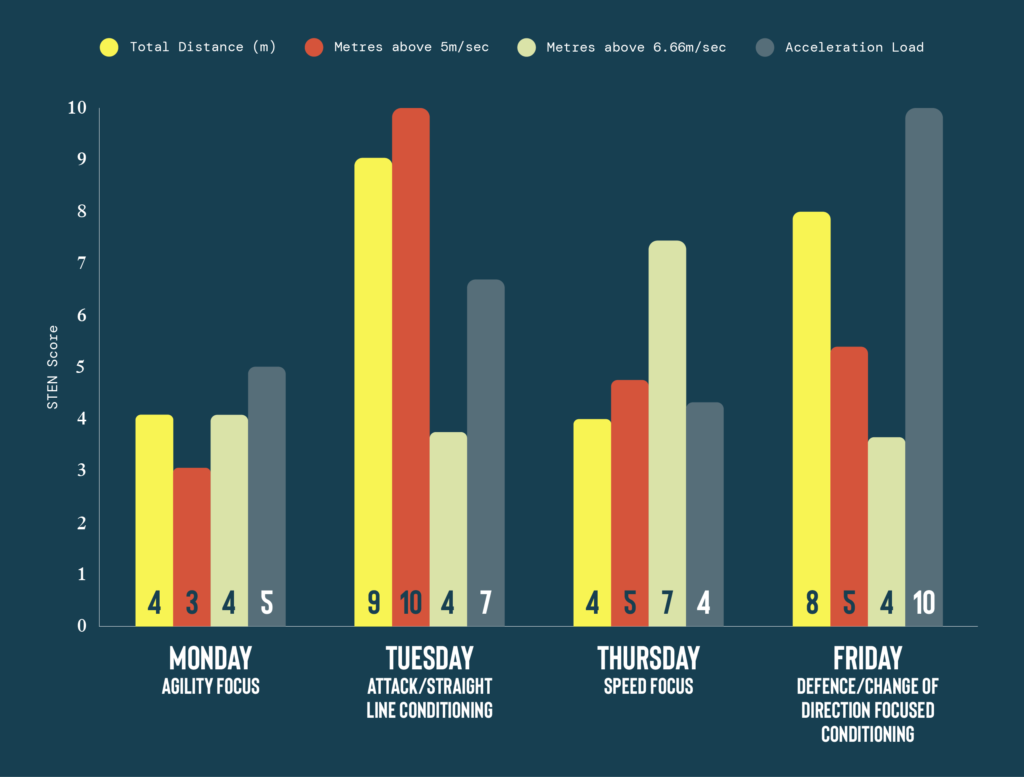
This illustrates how practitioners can vary the training stimuli across the training week to develop resilient athletes and avoid monotonous training.
Assess resilience by comparing internal and external variables
Tweet ThisPlanning training and monitoring responses are different. Comparing internal and external workloads provides insight into player fatigue and capacity, guiding effective training adjustments to build resilience.
@Billy_Hulin
Planning training and monitoring the response to training are two different concepts that require two different approaches. If your desire is to monitor and highlight when players may be experiencing some form of fatigue or gain a potential improvement in physical capacity, there is excellent research available on comparing internal and external workloads [21,22]. These studies provide the rationales and evidence for measures of external training load and how they relate to internal responses.
Comparing internal and external workloads will likely require different external workload variables to plan training.
Planning training should involve different types of workload, whereas global external workload is the consideration when making comparisons with the internal response. Therefore, variables such as overall accelerometer load, mechanical work, or metabolic work are preferable over isolated high speed running or acceleration demands [23,24]. External workload that considers body mass, speed, and acceleration is more strongly related with improvements in physical capacity than variables that do not take these factors into account [23].
During a training session in the early preseason, players have experienced high external demands that induced a high internal response (Figure 2, blue plots). However, over the course of a preseason, players should develop physical and mental adaptations, and become more resilient to external demands. This may lower their perceived exertion for the same external workload, which is the case for some players following a session in the late preseason (Figure 2, orange plots). Furthermore, when they taper their training before a competition, a lower external workload should align with lower internal response (Figure 2, green plots).
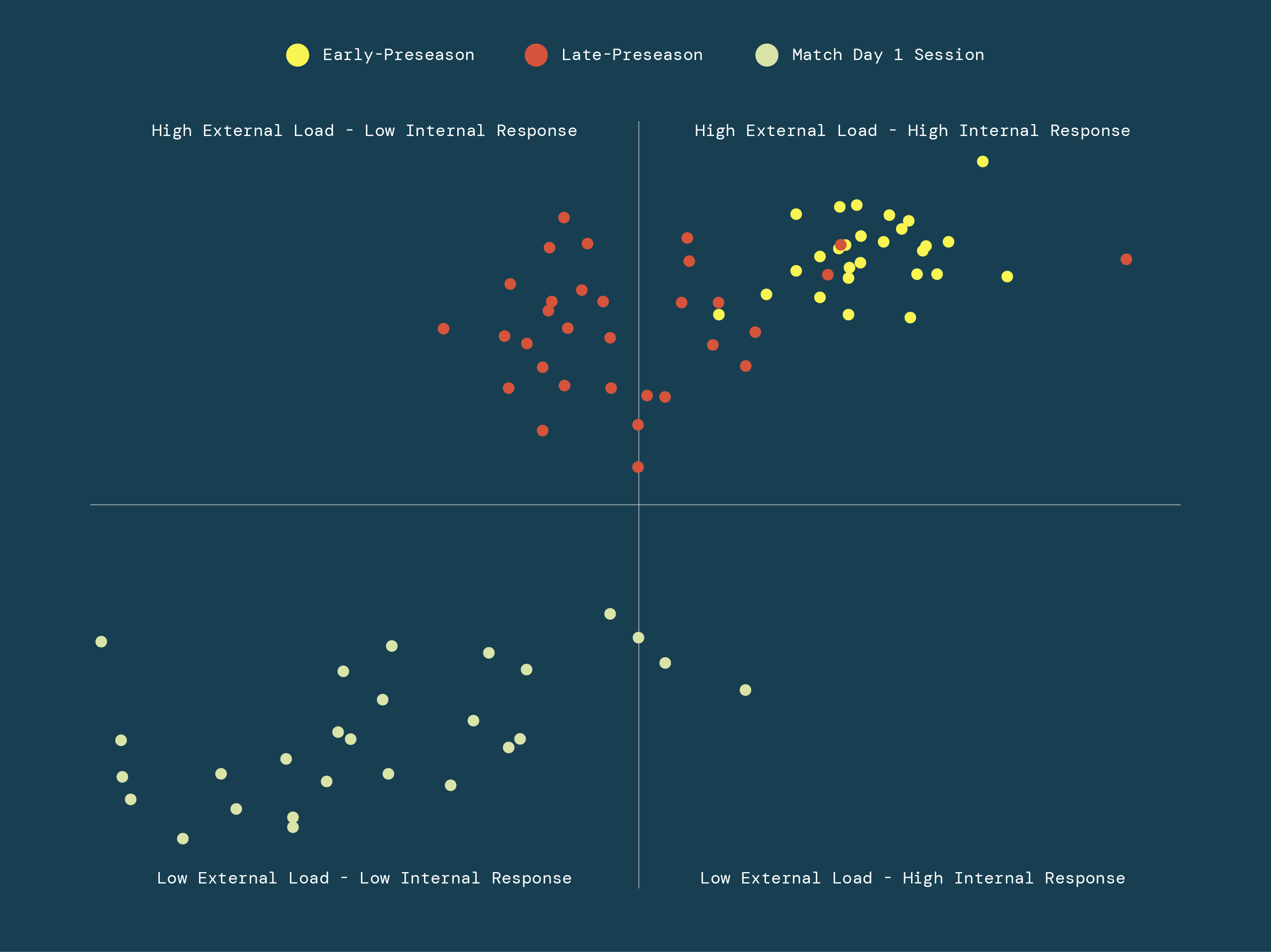
Figure 2. Example of comparing internal and external data. Individual z-score standardised versions of accelerometer derived workload and session rating of perceived exertion are on the vertical and horizontal axis, respectively.
The example in Figure 2 also shows how we can identify outlying players that may not have developed the desired adaptation or response to a program, which can drive further investigation into their individual circumstances.
These types of analyses are never perfect in an applied setting. Many confounding factors that cannot be included or measured will influence heart rate or perceived exertion. Practitioners have to acknowledge the uncertainty in this area and incorporate that into their planning for player development.
Prepare for every scenario, not the worst case scenario
Tweet ThisPreparing for every scenario, not just the worst case, means exceeding in-season demands during preseason. This builds resistance to high volumes of work, ensuring players can handle the stresses of a congested fixture schedule or playoff series.
@Billy_Hulin
The worst case scenario, in this context, is the maximum load or output in a specified time window [25]. Game based training that is above match intensity in a variety of epochs is essential to a good program in team sports. Many forms of training intensity are typically neglected or poorly designed in practice due to a myopic “how many kilometres did we do today?” focus on training volume.
But this perspective on “worst case scenario” is ambiguous and can not be applied in the same way with multiple variables.
A more productive approach is to devote specific parts of a main training session to training above match intensity, using variables that are relatively stable and reliable to quantify intensity. For example, the average intense five minute period during an Australian Football match may be approximately 155 m/min, or have an average acceleration of ~0.8 m/sec2 [26]. These, therefore, seem like reasonable targets for game based training drills that are five minutes long. Other metrics such as distance covered in various velocity bands (i.e. >5 or >7 m/sec) have too much variability between players and matches for practitioners to use them confidently in this fashion [25].

Nevertheless, during preseason players should still meet and exceed on a daily basis the in season running demands over set velocity thresholds. For example, if a player needs to cover 300 metres above 7 m/sec in a match and 500 metres over a seven day period, they should certainly be exceeding that workload on a daily and weekly basis on multiple occasions during preseason.
Focusing on short duration, high intensity periods alone may neglect other demands that players need to be prepared for, such as longer duration periods at 60-80% of the mean maximum one minute period of a match. For example, Australian Football players will cover ~85% of their total distance at a speed that is 30 – 80% of the peak one minute period of game [27]. A focus on only achieving peak intensity periods may neglect the lower intensity demands that require different energy system development and adaptations than short duration, high intensity efforts [28].
Depending on the goals of a specific session, training should regularly (but not always) aim to replicate the peak and submaximal demands of match play. The details of this type of training will depend on other confounding factors, such as the turnaround time between matches, the overall periodisation plan, or the other training content that coaches may wish to include within a session or week.
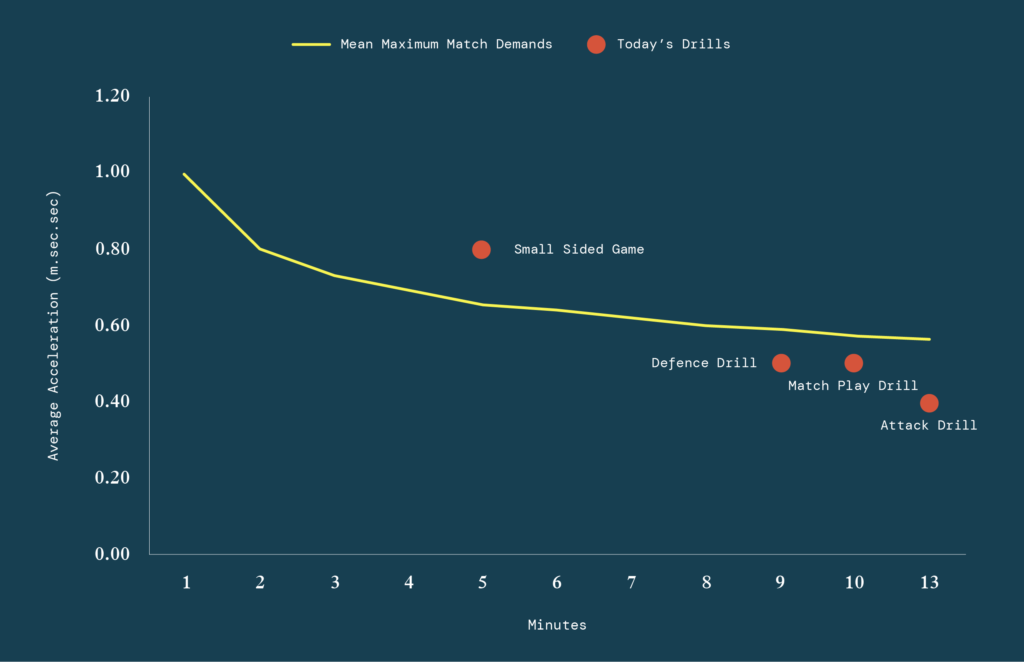
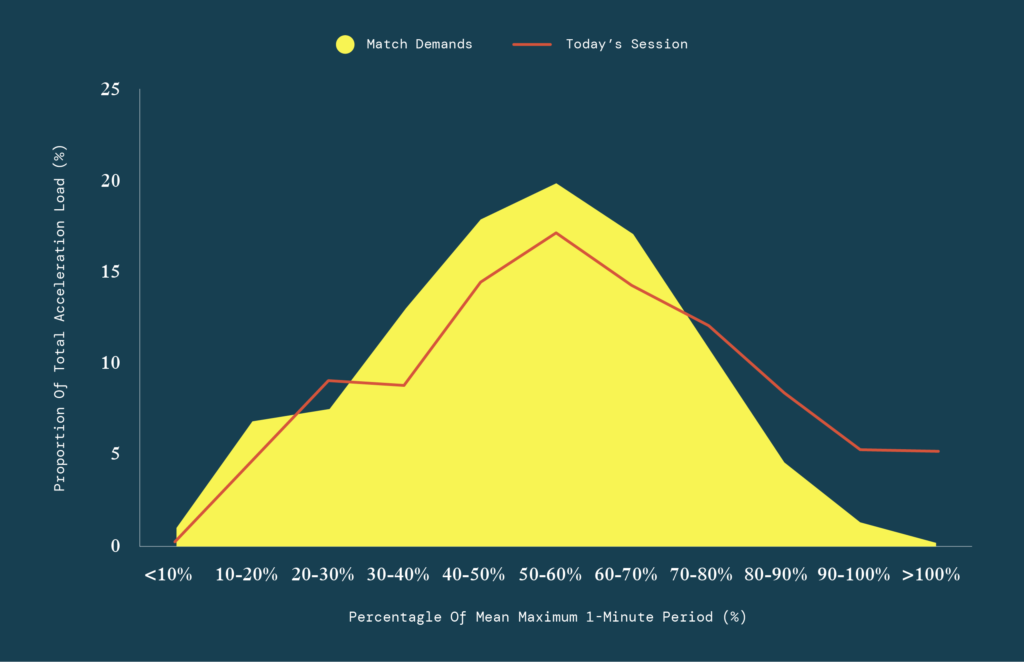
An example of a training session’s main drills in relation to the peak intensity average acceleration for specific epochs during matches are in Figure 3A.
Within this training session, the small sided game had significantly greater average acceleration than an intense five minute period of a match, which is excellent if your goal is to have a five minute period of “worst case scenario” training. However, viewing the session in its entirety in Figure 3B, there is a significantly smaller proportion of acceleration load between 30-70% mean maximal one minute peak period. Whether this is a good or bad outcome will depend on the training goals and the context of the session relative to the whole program over a micro- or mesocycle.
An actionable outcome from these data in Figure 3 may be crafting a subsequent session that provides a complementary dose of training, one that prepares players for the different ranges of intensity that they encounter during matches.
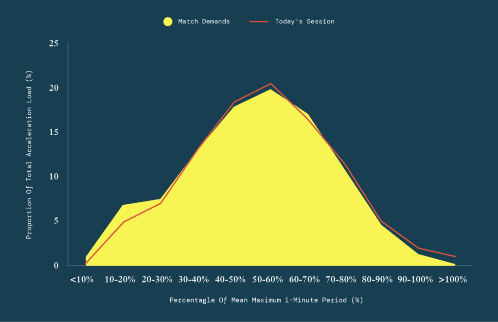
An example of a complementary training session is in Figure 4. No individual drill exceeds the mean maximum match demands for that specific time window (Figure 4A). However, the proportion of acceleration load at various intensities is very similar to matches, and slightly higher than a match at >90 and 100% of the mean maximum one minute period (Figure 4B).
These data do not say anything about the quality of this training session. Those evaluations will depend on the specific goals of the program and other training stimuli beyond what we are talking about here.
The information in Figures 3 and 4 merely highlights that training at match intensity is more complex than isolated periods or small sided games within a session or time window. Match specific conditioning can take many forms, and practitioners should always be open to assessing and reflecting on better ways to achieve these goals as technological advancements continue.

Be proactive with training volume to avoid reactive decisions
A proactive attitude to training monitoring and management would give some consideration to higher training and playing volumes that each player may encounter over a single day, a microcycle (roughly one week), and a mesocycle (e.g., 3-4 weeks). During preseason, players need to experience several different training parameters at a volume that is significantly greater than what might be considered “high” during in season. Figure 5 provides an example of visualising where a player’s current training volume is in relation to their average plus the interquartile range over an entire season during seven and 21 day timeframes. For example, a fully enclosed ring represents their current training volume equalling their average plus the interquartile range.
During preseason, these rings should be closed on multiple occasions. That way, when these situations occur during the season, players have some resistance to this volume of work.
Practitioners can accomplish this by using traditional periodisation strategies such as progressive overload during a preseason mesocycle. However, they should plan training in a way that allows players to reach volumes that exceed the demands of the season for different types of work.
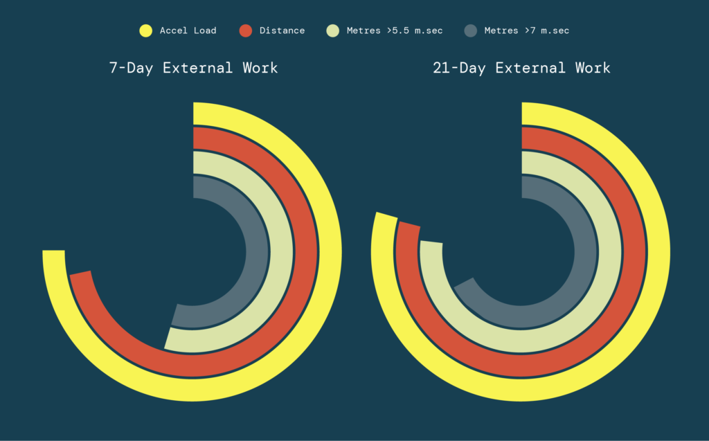
There is no perfect and certain way to manage training volume with complete accuracy. Figure 5 is close to an ideal scenario for a player the day before a few important occasions they may encounter during a season, such as a congested fixture period, a playoff series, or return to play from long term injury.
The player in Figure 5 has completed around 50-70% of a high seven day period and 70-80% of a high 21 day period, which represents a reduction over seven days and a good period of work in the 21 days prior to this milestone. This player is in a good position in terms of the volume of work they have completed. However, it is also important to consider whether the player has completed a high amount of work in the most recent months.
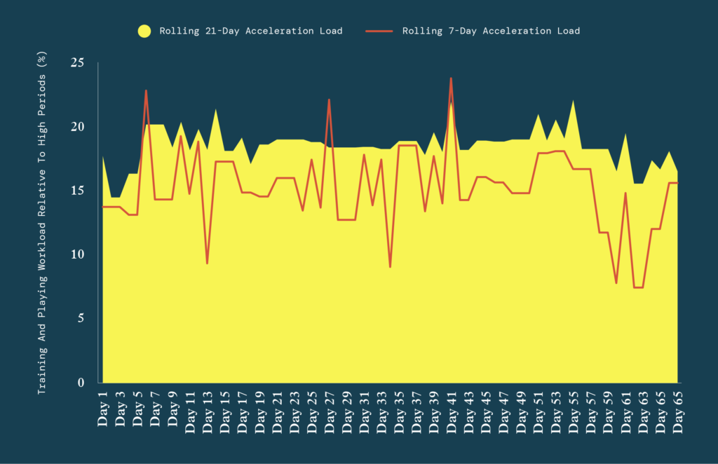
Figure 6 describes the same player’s acceleration load during the 67 days preceding this milestone. Figure 6 shows multiple key events that are important for developing players’ resilience in players. These include multiple exposure to high seven day workloads, several occasions of high 21 day workloads, a tapering or reduction in seven day workload the week prior to performance, and maintaining a 21 day workload that is greater than 80% of what might be considered high.