Using velocity based training to monitor training adaptation

Velocity based training conversations usually revolve around programming, which neglects how powerful VBT methods can be for monitoring adaptations. Changes in velocity at different loads give coaches new ways to measure success (potential positive adaptations occurring from the programming) and identify negative outcomes, e.g., fatigue or decreased neuromuscular readiness.

Expanding VBT usage to include this “invisible” type of monitoring should be pretty easy for anyone already collecting velocity data.

The first step is knowing the methods and metrics that may be useful for identifying and evaluating these changes. How much of a change in velocity is meaningful, under what circumstances, and what does it reflect?

As a simple example, the session to session, longitudinal change in an athlete’s load-velocity profile (LVP) or predicted 1RM could indicate if and how the athlete is changing over time. Coaches may compare the predicted values and ranges from the established minimal velocity threshold (MVT), or assess the intercept and slope of the regression. This is a relatively simplistic look at the data, but is a useful descriptive that a spreadsheet can surface quite easily.

Monitoring starts with establishing the reliability of the measures that we are using. A reliable measure will allow coaches or sport scientists to detect real changes, whereas a noisier measure will be more prone to errors and more difficult to detect change at all. Overall, performance practitioners should always be thinking about the reliability of the technology we use, especially when we are using it to determine if our interventions have been successful.

It can be challenging to investigate reliability as it requires a period of testing, preferably without any change in the “subjects.” That goes against everything we do as coaches – from Day 1 we are working to improve our athletes.

As a proxy, we can use data gathered by others in a controlled setting to get a sense of our technologies’ and methods’ reliability.

For example, Weakley et al ^[2] showed the Perch VBT device to be both valid and reliable for collecting velocity data in two compound exercises. Perch showed low bias within concentric mean velocity (~0.01 m/s) in both back squat and bench press across a range of loads 20-100% 1RM. They also calculated the standard error of measurement (SEM) and minimal detectable change (MDC) values across two testing sessions for each load. This gives us a going-in position for values that we could use to measure change in velocity for these exercises.

Despite the potential challenges, it’s still best practice to verify the reliability of your own data. Practitioners can attempt to replicate the methods of others to see if it leads to similar results. This process can be fairly simple, such as a test-retest or subsequent repeated measures design, using the same standardized procedures with a small period of time (one week or less).

Between-athlete test-retest reliability

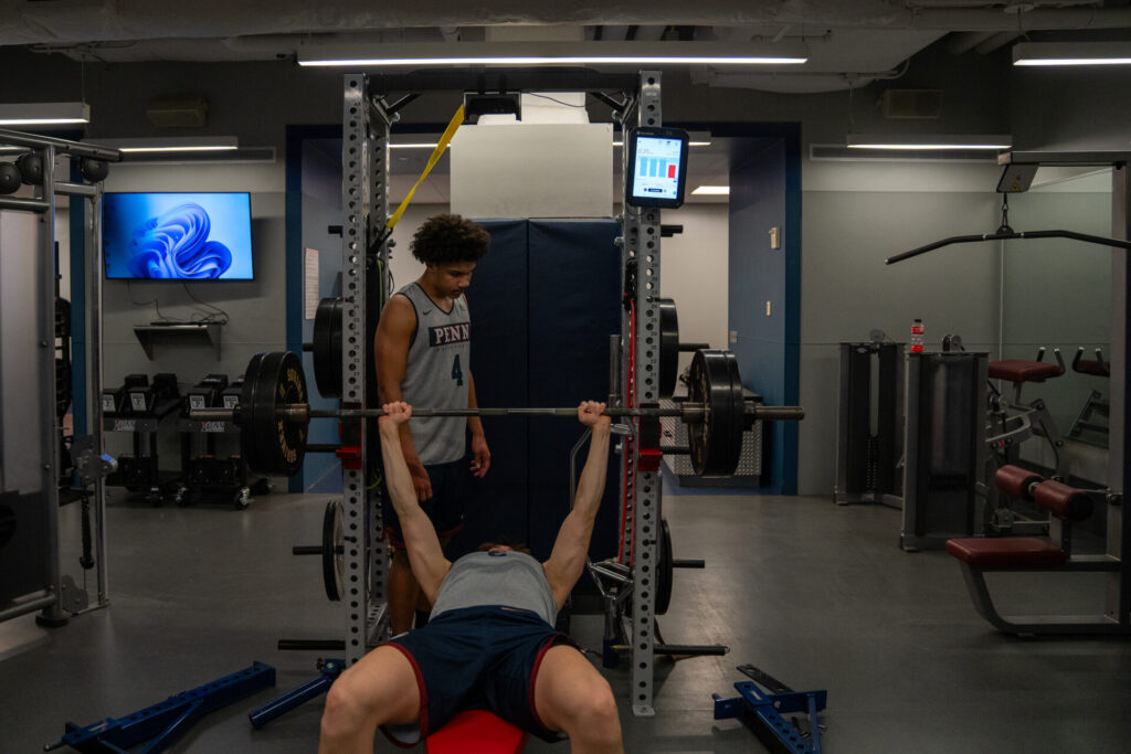
Sports performance does not permit us a “do nothing” block, so the start of a new phase (e.g. preseason or off season) generally is the best time to implement your internal reliability study.  Below is an example of a simple test-retest design during preseason. The athletes perform the target exercise (bench press at 185 lbs) seven days apart following the same lead up sequence of activities: an off day the day before, with no practice activities before performing the bench press.

A number of statistical approaches can test for reliability, including a comparison of difference scores, intraclass correlations and the mean square error from an ANOVA model.

Standard error of measurement is one of the most approachable. In the case of our data, this accounts for the variability introduced by both the technology and inherent variability of the athlete performing the test. Smaller values of SEM indicate less noise in the measure, suggesting a more stable measurement _[5].

Once we have an insight into the uncertainty surrounding our measure, we can understand what magnitude of change will suggest that it is a real and meaningful effect, and not just noise. That means we need to establish a practical threshold to assess a meaningful change ^[1].

Within your searches you may stumble across terms like smallest worthwhile change (SWC) scores, smallest detectable differences (SDD), minimal difference (MD), minimal important difference (MID), minimal clinically important difference (MCID) and so on. Each of these refer to a way of assessing the smallest change necessary to be practically relevant and not the product of chance.

The coach may ultimately determine this threshold based on their knowledge of what may be practically relevant to the sport. But, in some circumstances, we just may not know what changes to expect. When that happens, these statistical approaches provide a general sense of what values could support the change thresholds that can guide our decision making.

For example, a distribution based method that utilizes Cohen’s d against the baseline between-subject standard deviation (smallest worthwhile change =  SD_Basline * 0.2) suggests this value reflects the smallest effect needed to change performance scores. In our example, we see that the SWC and SEM are similar values. One may conclude that a ± 0.04 m/s change is real and practically meaningful. Another method is adding the SEM and SWC together to create a meaningful boundary with a higher probability that the change is real and meaningful. In the foregoing example, this would be ± 0.08 m/s.

Alternatively, other effect sizes could be appropriate, particularly in the case of a larger SEM, where you want SWC > SEM. Increasing the magnitude of the effect to moderate = SD_Basline * 0.5 and large = SD_Basline * 0.8 gives us values of 0.09 m/s and 0.14 m/s, respectively. This approach has given me my first general sense of the values that would guide my interpretation of changes in velocity. However, it’s important to note that these effect sizes are arbitrary and may not always be useful in all cases.

Alternatively, Weir ^[4] suggests using the minimal difference score calculated from the established SEM value of the test-retest. 

Within our example, MD = 0.1 m/s (for 90% CI) with a range of 0.08 m/s to 0.15 m/s. This can can vary with the confidence level: 0.08 m/s (0.06 – 0.11 m/s; 80% CI) or 0.12 m/s (0.09 – 0.19 m/s; 95% CI). Coaches can decide whether to be more or less conservative depending on their data. Weakley et al ^[1] use an 80% CI threshold within their examples, whereas Weir ^[4] uses a 95% CI threshold and Hopkins suggested 90% CI in his work ^[6].

I typically use a 90% CI, but there may be times where you use different thresholds based on the goal of your program. A larger interval has more precision and may be more suitable for off season responses, while a smaller interval is more sensitive changes and therefore will be more likely to produce a red flag in season. Setting a threshold too small may result in false positives, detecting every change every time you train, while too large of a threshold may not detect any changes at all (false negatives).

This group level approach works best with homogenous populations – athletes with similar characteristics in the same group – as a more diverse group may introduce higher between subject variability.

Observations from the within-athlete response

While the above approaches provide a group level means of estimating the variation and potential meaningful changes for velocity measures, they may be at times overly general and set changes beyond the meaningful range for the individual athlete.

For example, in basketball I have worked with point guards who have varied from 6’1” to 6’10”, 170 lbs to 245 lbs. Even if I used the above calculations accounting for a position group, there is still considerable heterogeneity within the group, which may lead to larger threshold values that are not applicable to each individual.

Therefore, a potentially more viable option is a method that calculates these measures at the individual athlete level. Using multiple observations on an individual we can estimate the within-subject standard error (SEM_within).

Weakley et al again provide an example ^[1] with charts illustrating how to assess whether an athlete changes over time. Excel is sufficient for replicating their methods.

We could use the observed break in trend (and subsequent new training block) to establish the new baseline. The positive trend from the subsequent four week training block (weeks 5-8) becomes the basis for assessing changes in the new training block starting at week 9.

Alternatively, the supplementary material of Weakley et al ^[1] mentions the “rule of 10”: 10 observations per single predictor in regression under similar conditions. In the case of this example, that would mean waiting 10 weeks to begin interpreting changes with this method. Again, that may be impractical for coaches who want – or need – to make decisions earlier in the process.

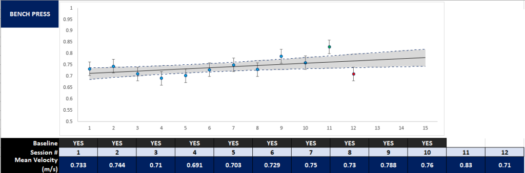
This approach is most reasonable for longitudinal trend analysis. However, another question here is if the threshold used is appropriate (0.3 * SD_within). This value comes from simulations of increasing the chances of theoretical medal placement in individual sports – not established changes in barbell velocity improving performance using this same approach. Nevertheless, it is still potentially a viable approach to monitor the primary trends in your data.

Setting anchors to detect meaningful changes

Some VBT research ^{[7, 8]}  suggests using a practical anchor to estimate the smallest effect size of interest (SESOI), using a load velocity profile (LVP) to perform these calculations.

These papers use a value of 2.5% and 5% 1RM to establish the minimal change in velocity to improve by the given percentage. This comes from multiplying the slope coefficient of the LVP by the given percentage of 1RM.

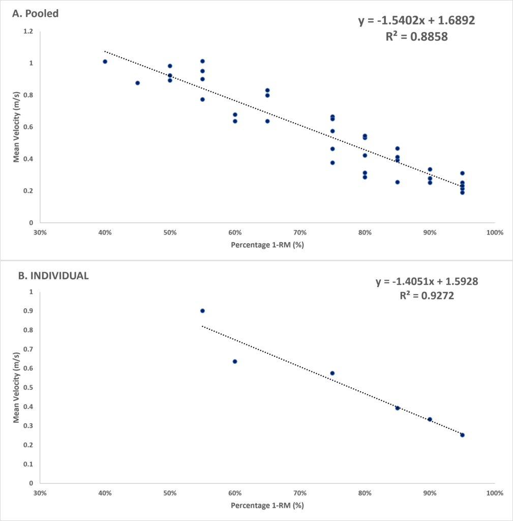
With both our grouped and individual profile examples, the SESOI can be calculated as the slope * 0.05: 1.5402 * 0.05 =  0.08 m/s, 1.405 * 0.05 = 0.07 m/s, for an average 5% change in percent 1RM.

Again, this gives coaches another fairly easy way to establish a potential practical threshold to measure whether a change has occurred in their velocity measure.

Combining approaches to determine thresholds for monitoring change

Each of these approaches offer slightly different estimates of potential values to assess the smallest meaningful changes in velocity measures. An approach I use is triangulating these values to understand what range of plausible values could establish change.

Suggested calculation	Values
Prior research [2] SEM = SDΔ / √☐ MD = SEM * CI * √☐	0.04 – 0.07 m/s   0.1 – 0.21 m/s
Internal reliability of between-subject test-retest SEM = SDΔ / √☐ SWC = SDBaseline * 0.2 SEM+SWC   SWCmoderate = SDBaseline * 0.5   SWClarge = SDBaseline * 0.8 MD = SEM * CI * √☐	0.04 m/s (0.03 – 0.06 m/s)   0.04 m/s   0.08 m/s   0.09 m/s   0.14 m/s   0.1 m/s (0.08 – 0.15 m/s)
Within-subject analysis of multiple observations SEMwithin √☐ SWCwithin = SDwithin * 0.3   SWCWithin + Baseline SEM	0.01 – 0.03 m/s (depending on baseline used)   0.01 m/s   0.02 – 0.05 m/s
Practical anchor based approach SESOI from pooled LVP: slope coefficient * 0.05   SESOI from individual LVP: slope coefficient * 0.05	0.08 m/s   0.07 m/s

The range of values stretches from 0.02 m/s up to 0.21 m/s. This is quite a wide range, with the largest observed values coming from prior research. Coaches have to decide which value(s) to apply to their data to assess change.

Taking into account all these values, the median is roughly 0.08 m/s and average is ~0.85 m/s. Therefore, this seems like a reasonable value and is covered in a number of our approaches: anchor based, the CI of the MD, SWC+SEM, and is roughly twice the SEM in the reliability example. Values above 0.08 m/s may be considered a meaningful change in our data.

However, I also use smaller and larger thresholds to give me a sense of some other plausible interpretations of the data.

We have our practical threshold of 0.08 m/s, which is the gray shaded area. We also have a smaller threshold, which is the SEM * 2; and a larger threshold, which is the MDC.

In this case, week 4 shows a drop in velocity below the smallest threshold we consider. This coincided with a four week overload period in which week 5 was a planned deload. The example showed an increase in velocity and break in trend of the data in week 6. However, in this example we interpret week 6 as being within the normal range given the average of weeks 1-4. Week 7, on the other hand, shows a potential change above the smallest threshold we could consider meaningful. But none of these values are greater than the gray shaded area, which may mean the athlete hasn’t changed at all during this training period for this given exercise.

What baseline is appropriate?

There is no best answer here, but the following approach has been useful within my reporting.

1. Longitudinal trend of all historical data within the season, monitored using the within-athlete response methods, with the trivial area representing a 90% CI around the forecasted baseline; or the approach recommended by Weakley et al ^[1].
2. Comparing to the previous training block. As the bigger phase progressions of the program generally follow from transitions in our season (preseason to competition, non-conference to conference competition, off season) I use the average of the previous block as a baseline for comparing the next block of training, assuming the exercise is in the next block. This can use both the raw values and the change scores assessed against your threshold test.
3. Assessing acute changes as the difference from week to week, resetting the baseline each week.

These are three methods to inform programming, providing a simplistic means to answer:

• How is an athlete changing over time?
• How is the current training block progressing relative to previous training blocks?
• What is the acute athlete response to this program?

VBT methods help practitioners monitor changes in their athletes and adjust their programs accordingly. This also helps us demonstrate our worth, by giving us reliable data showing how the athlete is progressing, while also alerting us to declines in performance related to fatigue or other factors that may affect an athlete’s readiness to perform.

Practitioners should use a combination of methods to determine a threshold for a meaningful change within the data, understanding that these thresholds are potential boundaries and not absolute values.

There is still much more to do in this space in terms of assessing what changes in velocity are meaningful to impact actual sports performance measures.