Enhancing force-velocity profiles with stride characteristics: Applications for performance and rehab

Applying certain areas of research to coaching practice are easier than others, such as maximal aerobic speed (MAS). But overall, speed is always a critical challenge. More accurately, measuring speed is easy but understanding what makes an individual fast certainly is not.

Force-velocity profiling has a myriad of applications both on the field and in the gym. However, on its own, F-v profiling is insufficient, even when we incorporated it into our Speed Signature methodology that I described in my previous article, The Speed Signature: A new way to understand “how” athletes run

Jurdan Mendiguchia ^[5–7] examined horizontal force profiles post-hamstring injury and demonstrated the importance of understanding changes with respect to injury risk and rehabilitation. Similarly, Matt Brughelli et al ^[8] extended the work of J-B Morin ^[3] by investigating intra-limb differences in athletes with hamstring injuries in Australian Rules Football. Research like this is critical in developing more informed programs for both injury prevention and rehabilitation. But there are two important things to take away from this work: changes in running gait persist after injury, and those changes can be identified between limbs.

Therefore, our next milestone is examining F-v in conjunction with individual limb data.

The approach we are taking is integrating ground contact time (GCT) and flight time (FT) with the F-v profile into the Speed Signature (Figure 1).

Figure 1. Top Panel: Speed-Time plot with GCT (grey bar + data) and FT (gap between grey bars). Red dashed line is actual velocity. Bottom Panel: Relative Horizontal Power-Time Plot with GCT (grey bar + data) and FT (gap between grey bars).

Ground contact time and flight time offer greater detail into the actions and capabilities of each limb. While we can’t measure force vectors per limb, information about GCT and FT gives coaches a great insight into what is happening per limb.

The data above shows a high agreement with 240fps video for both GCT and FT. We quantified this with a posterior density interval of 89% with a 0.9 probability mass, in addition to a correlation of r=0.9 (p.value = 0.005). However, there is a limitation to how accurate we can be with one accelerometer. A future direction is pooling steps and presenting variations across sessions, not individual steps, which exceeds the accuracy of the sensors.

Applying F-v profiles in conjunction with ground contact time

The following example is from a professional athlete eight months after a left ACL reconstruction.

When this athlete resumed accelerations, early sessions (Figure 2) showed that the left limb’s GCT was markedly lower than the right limb’s (highlighted by yellow lines).

This presentation contrasted with isokinetic testing and all single leg lifts in the gym, throughout which leg strength was bilaterally equal. This indicated that the athlete possessed the basic strength qualities but had lost the capacity to apply it in a task specific setting. That, in itself, reinforces what the research tells us: it doesn’t matter how strong you are in the gym, it’s what you apply to the ground in running that matters. It also highlights how strength exercises and tests we use in clinical or gym settings are specific only to the task they examine: jumping, hopping, isometric force tests, etc. From them, the most we can do is extrapolate an individual’s capability to run. Only a running-based test can provide an adequate foundation for assessing the athlete’s progress and progression. 

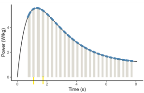
Figure 2. Early phase return to acceleration. Grey bars = GCT, Gaps = FT. Step 1-2 not graphed. Yellow bars highlight that left limb GCT is much faster than right limb.

Even without a deep dive into the data, we could still see that this athlete wasn’t accelerating correctly. He was getting off his left limb as quickly as possible and not “driving through” the high force, large GCT steps at the start of acceleration. His broader strategy was to get upright as fast as possible so he could “pull,” to borrow one of Stu McMillan’s descriptors. Incidentally, pulling is his default running “signature.”

Recognizing deficiencies and programming correctives

Based on these visual observations and the quantitative evidence of a low GCT on the reconstructed limb in early phase acceleration, I concluded that this athlete lacked the specificity to generate power during acceleration through the rehabbing limb during longer GCT – despite having adequate “strength” to do so.

To address this profile, we first added some light resistance work to his acceleration load. This was not to encourage greater force, although that was likely a secondary consequence. The aim was to coerce the athlete – using the constraint of additional load – into higher ground contact times.

To increase specificity of strength practice, I introduced a lift in the gym that matched his estimated GCT for the first three steps (~200-250 ms), then progressively increased the applied power to match what the athlete did on the field (Figure 3, red line). The constraints of the lift, therefore, were the timing and the relative power range indicated by on-field acceleration from the previous day. 

Figure 3 shows the athlete approximately three weeks after Figure 2. As the athlete improved, GCT equalised and he achieved far greater relative power during acceleration.

Figure 3. Late phase return to acceleration. Grey bars = GCT, Gaps = FT. Step 1-2 not graphed. Note the early symmetry in GCT and progressive reduction as speed increases. Red line highlights the estimate of relative power (w/kg) exerted in first two steps.

The lift the athlete and I favoured to achieve these goals was a modified single leg reverse lunge on a Smith machine. He started low, focusing on having the front (“drive”) limb as close to the angle required during the first three steps of acceleration.

While the Smith machine can be controversial, in this case it allowed 100% focus on power development with no concern for balance. Furthermore, the running data was based on horizontal power, while the lift is quite clearly vertical.

We acknowledged that this is not running and, while we try to get close as possible in a few respects, this type of work can never be 100% specific. On the scale of specificity, this was relatively low compared to the resisted acceleration work. That said, it is more specific than squatting or many other common alternatives. Equally, I felt that the quad and glute loading and contractile parameters were very similar to those of running, and they occurred in a movement pattern that was transferrable to running.

But more than anything else, the athlete was comfortable with the exercise and the program because he had input into what he was doing. That enabled him to bring the necessary intent and intensity.

Figure 4. Modified Smith machine reverse lunge. The athlete starts in an isometric hold (<2sec) and drives up on the front leg. It is critical that the hip, knee and ankle extend in sequence and the rear leg plays as little part in the drive phase as possible.

Additional parameters for profiling and programming

Weyand et. al. ^[1] noted that putting more force into the ground results in faster speeds. Too often, coaches interpret and operationalize this as: bigger squat = faster running. While increasing general strength can have a broad impact on running speed, specifically during acceleration, top speed takes more quality.

The change in vertical centre of mass velocity (CMV_V) is greater in faster athletes, which concurs with Weyand et al: more vertical force into the ground results in faster running (Figure 5a and Figure 5b). The athlete in Figure 5a has ~10% higher maximum speed, which is associated with ~16% greater CMV_V. This data enables the coach to figure out what lifts and drills contribute to the changes the athletes are experiencing as they develop and run faster.

Figure 5a. Y-axis: g_vert/kg. X-axis: left and right limb. Beige area = normative data. Athlete maximum speed ~9.8m/s

Figure 5b. Y-axis: g_vert/kg. X-axis: left and right limb. Beige area = normative data. Athlete maximum speed ~8.9m/s.

The other feature of this data is the asymmetry in the athlete in figure 4b. This likely contributes to his reduced maximum speed. Having this data available lets the coach not only recognize the asymmetry and investigate its root cause (e.g., a previous injury), but address the absolute deficit. Again, with an intervention in hand, this very specific maximum speed variable can be evaluated for progression.

Returning to the post-ACLR athlete mentioned above, he achieved his personal best maximum velocity around mid-April. During a session in mid-May, the plan was to get back up towards that speed after he had almost fully returned to team practice. The warm-up was great and there were no incidents during the session, but his maximum speed was off by quite a margin. Toward the end of the set, I noticed a slight lack of extension in the reconstructed knee while walking during a recovery period. This was odd, given the athlete had achieved full range of motion in the knee some time ago, and ROM restrictions did not appear anywhere in his medical review. On physical examination, the knee was lacking a few degrees of ROM.

The data clearly showed that his stride length relative to leg length on the reconstructed side (Figure 6, left = blue) had been impacted by the lack of knee extension and was well outside his normal range (beige shading) at 7-8 m/s. Reviewing the change over time of step length (Figure 6) confirmed a change in relative step length over time after the April 15 peak in speed and subsequent return to team training.

These observations suggested that the lack of ROM in the knee affected front side mechanics, and likely resulted in some loss of running skill during the return to team training. The end results were the measured change in step length and a lower maximal speed.

Figure 6. Relative step length vs. Speed. Red = right limb, blue = left limb. Large dots are for the session being investigated, small dots are data points from all previous sessions.

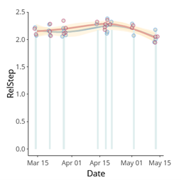
Figure 7. Relative step length change over time. Data is pooled in 1 m/s “buckets” and sampled from 8-9 m/s data. Red = right limb, Blue = left limb.

Despite having theoretically addressed knee ROM, we adapted the program to ensure the knee was mobilised before all high threshold activities. This athlete returned to personal best speed, and in the gym he improved his hop performance, another critical ACL rehab performance indicator.